The Activation Function

Part Zero - The Introduction

Part One - The Architecture Outline

Part Two - The Convolution Engine

Part Three - The Activation Function

Part Four - The Pooling Unit

Part Five - Adding fixed-point arithmetic to our design

Part Six - Putting it all together: The CNN Accelerator

Part Seven - System integration of the Convolution IP

Part Eight - Creating a multi-layer neural network in hardware.

Why do we need an activation function?

An activation function is a non-linear function that is introduced in order to realize a multi-layer neural network and not end up with a linear function. For the uninitiated, this article can be a good short introduction. A large variety of activation functions are used today but for the purpose of this article, we only implement the RELU function which at a point of time was the most commonly used one.

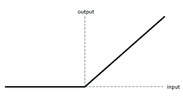
The following is a graph of the Relu activation function. Below that is the Verilog code implementing it.

NOTE: As the output of the RELU function varies based on the sign of the input, it can only be implemented in hardware when we start using signed numbers instead of just integers. However, the concept of positive and negative is only a mathematical concept on the software level. In hardware, there is no such thing as a negative number. Everything is just a register of a certain number of bits (32 in our case). However, the concepts like signed binary representation allow us to realize the concept of positive and negative numbers in hardware. Of course, another layer is necessary on top of the actual hardware in order to interpret the sign of these numbers and use them as required.

That layer has been written in python and shall be presented in the later stages of this series. Currently, we only look at the hardware architecture and Verilog code in order to keep things simple and get the bigger picture.

Implementing the ReLu function in Verilog

//file: relu.v
`timescale 1ns / 1ps
module relu(
    input [31:0] din_relu,
    output [31:0] dout_relu
    );
    assign dout_relu = (din_relu[31] == 0)? din_relu : 0;   //if the sign bit is high, send zero on the output else send the input
endmodule

Implementing Hyperbolic-Tangent in Verilog

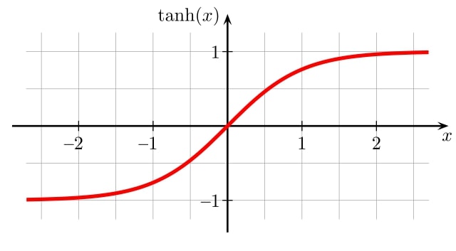
Tanh is another very popular and widely used activation function. It is just a scaled sigmoid and has some very useful properties. Here is a plot of this function:

We can implement such non-linear functions in several ways when it comes to hardware realization. For example:

• Simple Lookup Table, which happens to be the simplest and fastest way to realize a function but also takes up a lot of resources when a very high precision is required.
• Lookup Table with Interpolation, which is also a lookup table based method but uses a little bit of extra arithmetic to improve results beyond the precision being allotted for the lookup table itself. There are also methods that use two lookup tables, one with coarse grained values, and another with fine grained values which get added on to the initial approximation.
• CORDIC, this is another extremely popular method that is widely used in most DSP applications that need non-linear functions like, sine, sqrt, tanh etc. It is a very elegant method that uses basic shift-add circuitry to achieve very good results. You can read this post for a good implementation of CORDIC. Most FPGA vendors also provide packaged IP blocks for CORDIC units.
• Taylor series and polynomial approximations, these methods use the traditional polynomial approximations of trigonometric functions and try to implement the higher order variables in those polynomial.
• DCT Interpolation and more sophisticated methods, the methods use more specialized ways to achieve the exact precision and resource usage required.This paper shows one such method.

In this article, we shall be using the first two methods, i.e simple table lookup and a lookup table + interpolation strategy to get the tanh function. I shall be attempting the CORDIC method too in a future article.

Simple table Lookup

• For this implementation, we can exploit the symmetry of the Tanh function, i.e we only have to store the values pertaining to the positive side of the function and since the function output for negative inputs is just the mirror image, we can output the same values in their 2's complement format.
• One more property that we can easily exploit is the fact that the Tanh function saturates to 1 (or -1 on the other side) beyond a certain input value. Without any significant loss in accuracy, we can directly output 1 (or -1) for the inputs above a threshold. So we do not have to store the function values in the lookup table for inputs above a threshold. I'm using the input value 3 ( or -3) as this threshold since tanh(3) = 0.9950547536867305 and for all inputs above 3 (or below -3) the output can be comfortably be considered to be 1 (or -1).

• For this implementation I'm using a RAM with 1024 locations each holding 16 bit data in order to implement the lookup table. Which mean we shall have 10 (= log2(1024)) address bits to access this ram. But our phase input is going to be a 16 bit fixed point number. So how do we choose 10 particular bits to address this ram?

  Here is a sample 16- bit fixed point input in the (3,12) format to the tanh function:

  reg [15:0] phase = 16'b0_001_011000100101

  in this,

  • the MSB ( phase[15] ) is the sign bit, which will tell us whether to output the direct value or the 2's complemented form.
  • the next three MSB's represent the integer part of this number. Since we're only worried about the numbers whose magnitude is less than 3, if the second MSB ( phase[14] ) is high (for a positive number that is), it tells us that the magnitude of this number is above 3 and we can directly output 1 . Else, we can output the value from the table.
  • the next 10 MSBs ( phase [13:4] ) will be used as inputs to the lookup table. Yes we're going to lose the information in the LSBs ( phase[3:0] ) but if we wanted to use them too, we'd need a lookup table that's 16 times larger. As long as we're getting reasonable accuracy for our application, we need not worry. Further down we'll look at one technique that makes use of these LSBs as well.

  Here is the code for this implementation:

    `timescale 1ns / 1ps
    module tanh_lut #(
        parameter AW = 10, //AW will be based on the size of the ROM we can afford in our design.
                           //in the best case AW = N;
        parameter DW = 16,
        parameter N = 16,
        parameter Q = 12
        )(
        input clk,
        input [AW-1:0] phase,
        output [DW-1:0] tanh
       );
     reg [AW-1:0] addr_reg;
  (* ram_style = "block" *)reg [DW-1:0] mem [1<<AW-1:0];  //ram_style can be 'block' or 'distributed' 									                    // based on the utilization and other
                                                          //requirements in the project
    initial 
    begin
        $readmemb("tanh_data.mem",mem); //loading data into our RAM via a file
    end
        
    always@(posedge clk)
    begin
        addr_reg <= phase[AW-1:0];
    end
        
    assign tanh = mem[addr_reg];

Lookup table with linear interpolation

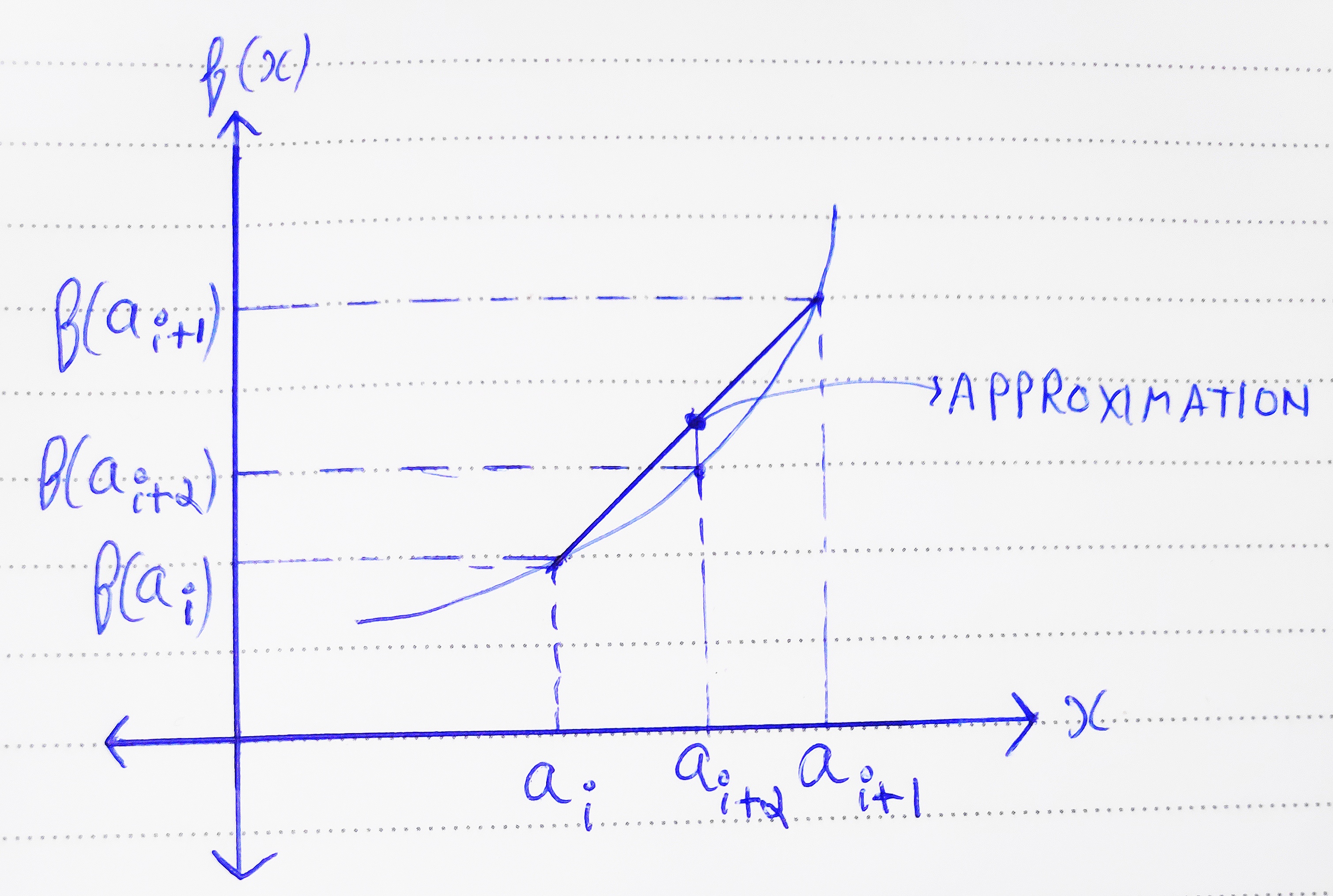
The linear interpolation technique is a commonly used trick in mathematics to improve the approximation of a value when not enough resolution is present in the data. i.e when you want the value of a discrete function between two successive data points, you can draw a straight line joining these two points and approximate your output to be somewhere on that line. This significantly improves the accuracy of our function.

Now, to explain this idea, take a look at the above image. Let's say a_i and a_i+1 are two consecutive points where we know the value of our function f(a_i) and f(a_i+1) . That is, in our case, these are two entries in our RAM for the value of Tanh at two consecutive points.

Let's say we want to find the value of the function at a point a_i+α where α is a fractional value less than one. This tells us that we need the value of f(x) between two known points, since we have no information on the actual shape of the curve in between these two points, one way to approximate this would be to assume a straight line between the two known points. By using basic linear mathematics, we can find out the value of the point on that straight line corresponding to x = a_i+α .

As you can guess, this approximated value will be f(a_i) + x( (f(a_i+1) - a_i)/1 ) = xf(a_i) + (1-x)f(a_i+1) and the error produced would be xf(a_i) + (1-x)f(a_i+1) - f(a_i+α)

This result would be relatively more accurate than the initial approximation from the lookup table. The value of α in our case will be derived from the remaining 4 LSBs that were ignored in the actual lookup table. Below is the code for this approach:

Note: I'm writing the code for a 16 bit wide data path. i.e N = 16 if you've been reading the other articles in this series. However, it can very much be parameterized to work with any bit width.

`timescale 1ns / 1ps
module tanh_lut #(
    parameter AW = 10, //AW will be based on the size of the ROM we can afford in our design.
                       //in the best case AW = N;
    parameter DW = 16,
    parameter N = 16,
    parameter Q = 12
    )(
    input clk,
    input [N-1:0] phase,
    output [DW-1:0] tanh
    );
    
    reg [9:0] addra_reg;
    reg [9:0] addrb_reg;
    wire [15:0] tanha;
    wire [15:0] tanhb;
    wire ovr1,ovr2;

    wire [15:0] frac,one_minus_frac;
    wire [15:0] A1,A2;
    wire [15:0] one;
    wire [DW-1:0] tanh_temp;

    
    (* ram_style = "block" *)reg [15:0] mem [1<<10-1:0];  //ram_style can be 'block' or 'distributed' based on the
                                                            //utilization and other requirements in the project
    
    initial 
    begin
        $readmemb("tanh_data.mem",mem); //loading our RAM via a file
    end
    
    always@(posedge clk)
    begin
        addra_reg <= phase[9:0];
        addrb_reg <= phase[9:0] + 1'b1;
    end

    assign tanha = mem[addra_reg];
    assign tanhb = mem[addrb_reg];
    
    assign frac = {'d0,phase[N-AW-'d2-1:0]}; //rest of the LSBs that were not accounted for owing to the limited ROM size
    assign one = 16'b0001000000000000;       //'d1 in (N,Q) = (3,12) format
    assign one_minus_frac = one - frac;
    
    //qmult is the fixed point multiplier module, visit the fixed point arithmetic
    //article further in the series to learn of its exact operation
    qmult #(N,Q) mul1 (tanha,frac,A1,ovr1);              //calculates x*f(Ai)
    qmult #(N,Q) mul2 (tanhb,one_minus_frac,A2,ovr2);    //calculates (1-x)*f(Ai+1)
    
    assign tanh_temp = A1 + A2;    // linear interpolation formula: x*Ai + (1-x)*Ai+1
    
    //now, if the phase input is above 3 or below -3 then we just output 1, otherwise we output the calculated value
    //we also check for the sign, if the phase is negative, we return 2's complemented version of the calculated value
    assign tanh = (phase [N-1]) ? (phase[N-2] ? (16'b1111000000000000) : (~tanh_temp + 1'b1)) :(phase[N-2] ? (16'b0001000000000000):(tanh_temp));
    
endmodule

All the design files along with their test benches can be found at the Github Repo

PREVIOUS:The convolution engine
NEXT :The pooling unit