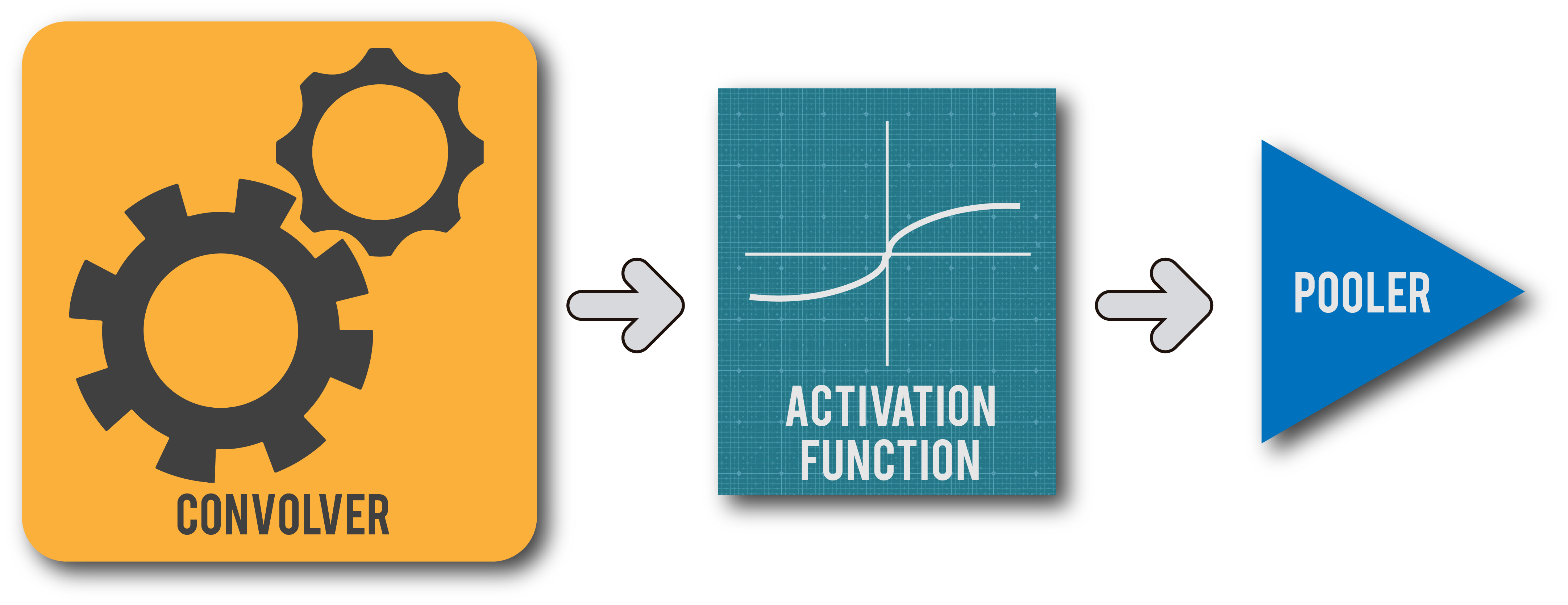
Putting it all together: The CNN accelerator

In this article, we put all the modules that we've designed in this series together and build a single unit of a CNN architecture.
Part Zero - The Introduction
Part One - The Architecture Outline
Part Two - The Convolution Engine
Part Three - The Activation Function
Part Four - The Pooling Unit
Part Five - Adding fixed-point arithmetic to our design
Part Six - Putting it all together: The CNN Accelerator
Part Seven - System integration of the Convolution IP
Part Eight - Creating a multi-layer neural network in hardware.
We finally have all the building blocks needed to build this accelerator (or at least a single layer of it) . In this post we're going to put all the layers that we've built together and wonder at the awesomeness of what we've built. Let's take a look at the code!
The Golden Model
First, we need a golden model that we can use to verify our digital design against, as usual, python is our friend. Let's take a look at it.
  1
  2
  3
  4
  5
  6
  7
  8
  9
 10
 11
 12
 13
 14
 15
 16
 17
 18
 19
 20
 21
 22
 23
 24
 25
 26
 27
 28
 29
 30
 31
 32
 33
 34
 35
 36
 37
 38
 39
 40
 41
 42
 43
 44
 45
 46
 47
 48
 49
 50
 51
 52
 53
 54
 55
 56
 57
 58
 59
 60
 61
 62
 63
 64
 65
 66
 67
 68
 69
 70
 71
 72
 73
 74
 75
 76
 77
 78
 79
 80
 81
 82
 83
 84
 85
 86
 87
 88
 89
 90
 91
 92
 93
 94
 95
 96
 97
 98
 99
100
101
102
103
104
105
106
107
108
109
110
111
112
113
114
115
116 | import numpy as np
from scipy import signal
import subprocess
import os
import math
import skimage.measure
from numpy.random import seed
#Function to convert from the Fixed point precision that our hardware is using to the float values that python actually uses
def fp_to_float(s,integer_precision,fraction_precision): #s = input binary string
number = 0.0
i = integer_precision - 1
j = 0
if(s[0] == '1'):
s_complemented = twos_comp((s[1:]),integer_precision,fraction_precision)
else:
s_complemented = s[1:]
while(j != integer_precision + fraction_precision -1):
number += int(s_complemented[j])*(2**i)
i -= 1
j += 1
if(s[0] == '1'):
return (-1)*number
else:
return number
#Function to convert between the actual float values and the fixed point values in the particular
#precision that our hardware is using
def float_to_fp(num,integer_precision,fraction_precision):
if(num<0):
sign_bit = 1 #sign bit is 1 for negative numbers in 2's complement #representation
num = -1*num
else:
sign_bit = 0
precision = '0'+ str(integer_precision) + 'b'
integral_part = format(int(num),precision)
fractional_part_f = num - int(num)
fractional_part = []
for i in range(fraction_precision):
d = fractional_part_f*2
fractional_part_f = d -int(d)
fractional_part.append(int(d))
fraction_string = ''.join(str(e) for e in fractional_part)
if(sign_bit == 1):
binary = str(sign_bit) + twos_comp(integral_part + fraction_string,integer_precision,fraction_precision)
else:
binary = str(sign_bit) + integral_part+fraction_string
return str(binary)
#Function to calculate 2's complement of a binary number
def twos_comp(val,integer_precision,fraction_precision):
flipped = ''.join(str(1-int(x))for x in val)
length = '0' + str(integer_precision+fraction_precision) + 'b'
bin_literal = format((int(flipped,2)+1),length)
return bin_literal
#Function to perform convolution between an input array and a filter array
def strideConv(arr, arr2, s):
return signal.convolve2d(arr, arr2[::-1, ::-1], mode='valid')[::s, ::s]
#setting random seed values for each call to random.uniform
seed(17)
#numpy array representing the input activation map
values = np.random.uniform(-1,1,36).reshape((6,6))
seed(2)
#numpy array representing the kernel of weights
weights = np.random.uniform(-1,1,9).reshape((3,3))
#2-D Convolution operation
conv = strideConv(values,weights,1)
#Activation function (alternatively this can be replaced by the Tanh function)
conv_relu = np.maximum(conv,0)
#Pooling function (alternatively np.max can be used as the last argument for max pooling)
pool = skimage.measure.block_reduce(conv_relu, (2,2), np.average)
#Converting all our arrays into the fixed point format of our choice to feed it to hardware
for a in values:
for b in a:
values_fp.append(float_to_fp(b, 3, 12))
values_fp_reshaped = np.reshape(values_fp,(6,6))
print('\nvalues')
print(values)
print(values_fp_reshaped)
for a in weights:
for b in a:
weights_fp.append(float_to_fp(b, 3, 12))
weights_fp = np.reshape(weights_fp,(3,3))
print('\nweights')
print(weights)
print(weights_fp)
for a in conv:
for b in a:
conv_fp.append(float_to_fp(b, 3, 12))
conv_fp = np.reshape(conv_fp,(4,4))
print('\nconvolved output')
print(conv)
print(conv_fp)
for a in conv_relu:
for b in a:
conv_relu_fp.append(float_to_fp(b, 3, 12))
conv_fp = np.reshape(conv_fp,(4,4))
print('\n relu conv')
print(conv_relu)
print(conv_relu_fp)
for x in pool:
for y in x:
pool_fp.append(float_to_fp(y, 3, 12))
pool_fp = np.reshape(pool_fp,(2,2))
print('\npooled output')
print(pool)
print(pool_fp)
|
The output of the above golden model looks something like this:
 1
 2
 3
 4
 5
 6
 7
 8
 9
10
11
12
13
14
15
16
17
18
19
20
21
22
23
24
25
26
27
28
29
30
31
32
33
34
35
36
37
38
39
40
41
42
43
44
45
46
47
48
49
50
51
52
53
54 | values
[[-0.41066999 0.06117351 -0.61695843 -0.86419928 0.57397092 0.31266704]
[ 0.27504179 0.15120579 -0.92187417 -0.28437279 0.89136637 -0.87991064]
[ 0.72808421 0.75458105 -0.89761267 0.30483723 0.10350274 0.19502651]
[-0.03294275 -0.43402368 -0.40454856 0.12301781 -0.20790513 0.57740142]
[-0.16303123 -0.71219216 -0.69818661 -0.8895173 0.43607439 -0.41536529]
[-0.60245226 0.66272784 0.13598224 -0.8353205 0.08999715 -0.68208251]]
[['1111100101101110' '0000000011111010' '1111011000100001'
'1111001000101101' '0000100100101110' '0000010100000000']
['0000010001100110' '0000001001101011' '1111000101000001'
'1111101101110100' '0000111001000011' '1111000111101100']
['0000101110100110' '0000110000010010' '1111000110100100'
'0000010011100000' '0000000110100111' '0000001100011110']
['1111111101111010' '1111100100001111' '1111100110000111'
'0000000111110111' '1111110010101101' '0000100100111101']
['1111110101100101' '1111010010011011' '1111010011010101'
'1111000111000101' '0000011011111010' '1111100101011011']
['1111011001011101' '0000101010011010' '0000001000101100'
'1111001010100011' '0000000101110000' '1111010100010111']]
weights
[[-0.1280102 -0.94814754 0.09932496]
[-0.12935521 -0.1592644 -0.33933036]
[-0.59070273 0.23854193 -0.40069065]]
[['1111110111110100' '1111000011010101' '0000000110010110']
['1111110111101111' '1111110101110100' '1111101010010011']
['1111011010001101' '0000001111010001' '1111100110010111']]
convolved output
[[ 0.29603207 -0.06693776 1.37891319 -0.44264833]
[-0.10188546 0.87896483 0.86022961 -1.3718567 ]
[-0.48097811 1.47415119 -0.03505743 0.49937723]
[ 1.20645719 0.93217962 -0.31713869 1.21348448]]
[['0000010010111100' '1111111011101110' '0001011000010000'
'1111100011101011']
['1111111001011111' '0000111000010000' '0000110111000011'
'1110101000001101']
['1111100001001110' '0001011110010110' '1111111101110001'
'0000011111111101']
['0001001101001101' '0000111011101010' '1111101011101101'
'0001001101101010']]
relu conv
[[0.29603207 0. 1.37891319 0. ]
[0. 0.87896483 0.86022961 0. ]
[0. 1.47415119 0. 0.49937723]
[1.20645719 0.93217962 0. 1.21348448]]
['0000010010111100', '0000000000000000', '0001011000010000', '0000000000000000', '0000000000000000', '0000111000010000', '0000110111000011', '0000000000000000', '0000000000000000', '0001011110010110', '0000000000000000', '0000011111111101', '0001001101001101', '0000111011101010', '0000000000000000', '0001001101101010']
pooled output
[[0.29374922 0.5597857 ]
[0.903197 0.42821543]]
[['0000010010110011' '0000100011110100']
['0000111001110011' '0000011011011001']]
|
The Verilog Module
Now that we have a solid golden model to guide us, let's look at the code for the actual module in Verilog.
 1
 2
 3
 4
 5
 6
 7
 8
 9
10
11
12
13
14
15
16
17
18
19
20
21
22
23
24
25
26
27
28
29
30
31
32
33
34
35
36
37
38
39
40
41
42
43
44
45
46
47
48
49
50
51
52
53
54
55
56
57
58
59
60
61
62
63
64
65
66
67
68
69
70
71
72
73
74
75 | //file:accelerator.v
`timescale 1ns / 1ps
`define FIXED_POINT 1 //This verilog macro tells the tools whether to instantiate a normal //multiplier or a Fixed point multiplier.
module acclerator #(
parameter n = 9'h00a, //size of the input image/activation map
parameter k = 9'h003, //size of the convolution window
parameter p = 9'h002, //size of the pooling window
parameter s = 1, //stride value during convolution
parameter ptype = 1, //0 => average pooling , 1 => max_pooling
parameter act_type = 0,//0 => ReLu activation function, 1=> Hyperbolic tangent activation function
parameter N = 16, //Bit width of activations and weights (total datapath width)
parameter Q = 12, //Number of fractional bits in case of fixed point representation
parameter AW = 10, //Needed in case of tanh activation function to set the size or ROM
parameter DW = 16, //Datapath width = N
parameter p_sqr_inv = 16'b0000010000000000 // = 1/p**2 in the (N,Q) format being used currently
)(
input clk,
input global_rst,
input ce,
input [15:0] activation,
input [(k*k)*16-1:0] weight1,
output [15:0] data_out,
output valid_op,
output end_op
);
wire [N-1:0] conv_op;
wire valid_conv,end_conv;
wire valid_ip;
wire [N-1:0] relu_op;
wire [N-1:0] tanh_op;
wire [N-1:0] pooler_ip;
wire [N-1:0] pooler_op;
reg [N-1:0] pooler_op_reg;
convolver #(.n(n),.k(k),.s(s),.N(N),.Q(Q)) conv( //Convolution engine
.clk(clk),
.ce(ce),
.weight1(weight1),
.global_rst(global_rst),
.activation(activation),
.conv_op(conv_op),
.end_conv(end_conv),
.valid_conv(valid_conv)
);
assign valid_ip = valid_conv && (!end_conv);
relu #(.N(N)) act( // ReLu Activation function
.din_relu(conv_op),
.dout_relu(relu_op)
);
tanh_normal #(.AW(AW),.DW(DW),.N(N),.Q(Q)) tanh( //Hyperbolic Tangent Activation function
.clk(clk),
.rst(global_rst),
.phase(conv_op[N-1:N-10]),
.tanh(tanh_op)
);
assign pooler_ip = act_type ? tanh_op : relu_op; //alternatively you could use macros to save //resources when using ReLu
pooler #(.N(N),.Q(Q),.m(n-k+1),.p(p),.ptype(ptype),.p_sqr_inv(p_sqr_inv)) pool( //Pooling Unit
.clk(clk),
.ce(valid_ip),
.master_rst(global_rst),
.data_in(pooler_ip),
.data_out(pooler_op),
.valid_op(valid_op),
.end_op(end_op)
);
assign data_out = pooler_op;
endmodule
|
Let's run our module with the above input activations and weights with the following set configuration parameters in the testbench:
| parameter n = 9'h006, //size of the input image/activation map
parameter k = 9'h003, //size of the convolution window
parameter p = 9'h002, //size of the pooling window
parameter s = 1, //stride value during convolution
parameter ptype = 0, //0 => average pooling , 1 => max_pooling
parameter act_type = 0,//0 => ReLu activation function, 1=> Hyperbolic tangent activation //function
parameter N = 16, //Bit width of activations and weights (total datapath width)
parameter Q = 12, //Number of fractional bits in case of fixed point representation
parameter AW = 10, //Needed in case of tanh activation function to set the size or ROM
parameter DW = 16, //Datapath width = N
parameter p_sqr_inv = 16'b0000010000000000 //1/4 in (3,12) format
|

We can see how the valid_op signal goes high only for 4 values of the acclerator output (acc_op) as expected. Also, plugging each of these values into the fp_to_float() python function above will tell you that the values are almost (although not exact due to precision loss) the same as those generated by the golden model. You can use the testbench to check the functionality for all the possible configuration parameters. However, we'll be looking at automating that tedious process in the next article.
All the design files along with their test benches can be found at the Github Repo
PREVIOUS:The architecture outline
